Some of my Experiences with Kalman Filters

Ronald Yannone

When I first started working at General Electric Company in Utica, NY in 1976, I had the opportunity to code up a Kalman filter for a target tracking application in BASIC programming language. Since that first experience, I was in love with the Kalman filter and have designed many for a variety of military applications since. In this introductory article I would like to share some of my experiences with Kalman filter design over the past 20 years.

R. Kalman put out the first article in 1960. A Kalman filter is simply an optimal recursive data processing algorithm. There are many ways of defining optimal, dependent upon the criteria chosen to evaluate performance. One aspect of this optimality is that the Kalman filter incorporates all information that can be provided to it. It processes all available measurements, regardless of their precision, to estimate the current value of all the variables of interest, with the use of (1) knowledge of the system and measurement device dynarnics, (2) the statistical description of the system noises, measurement errors, and uncertainty in the dynamics models, and (3) any available information about initial conditions of the variables of interest.

The word recursive means that, unlike certain data processing concepts, the Kalman filter does not require all previous data to be kept in storage and reprocessed every time a new measurement is taken. The "filter" is actually a data processing algorithm. Despite the typical connotation of a filter as a "black box" containing electrical networks, the fact is that in most practical applications, the "filter" is just a computer program in the central processor. As such, it inherently incorporates discrete time measurement samples rather than continuous time inputs.

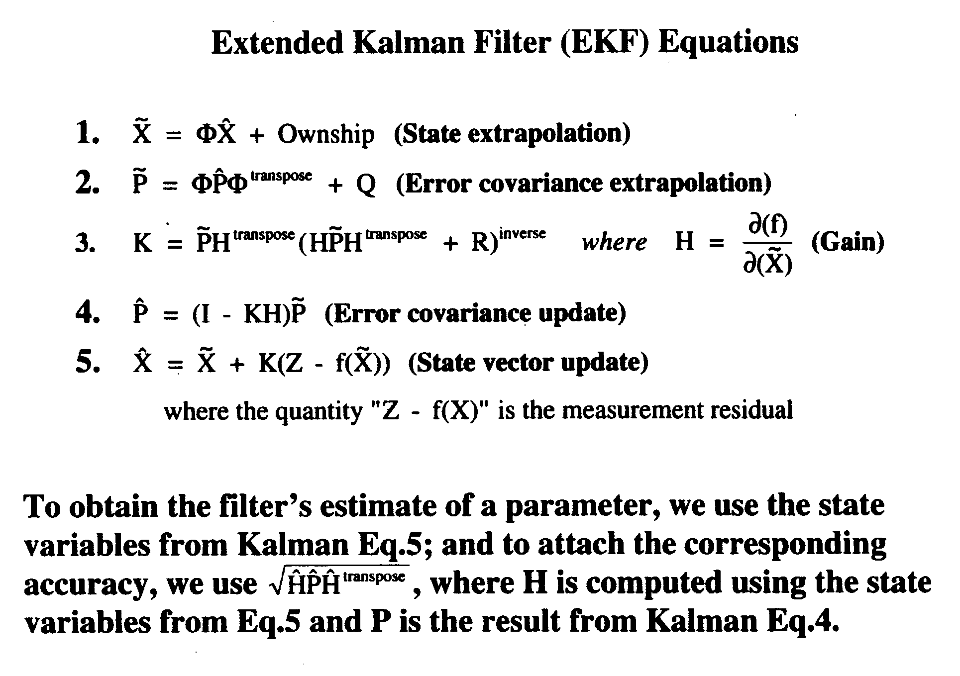
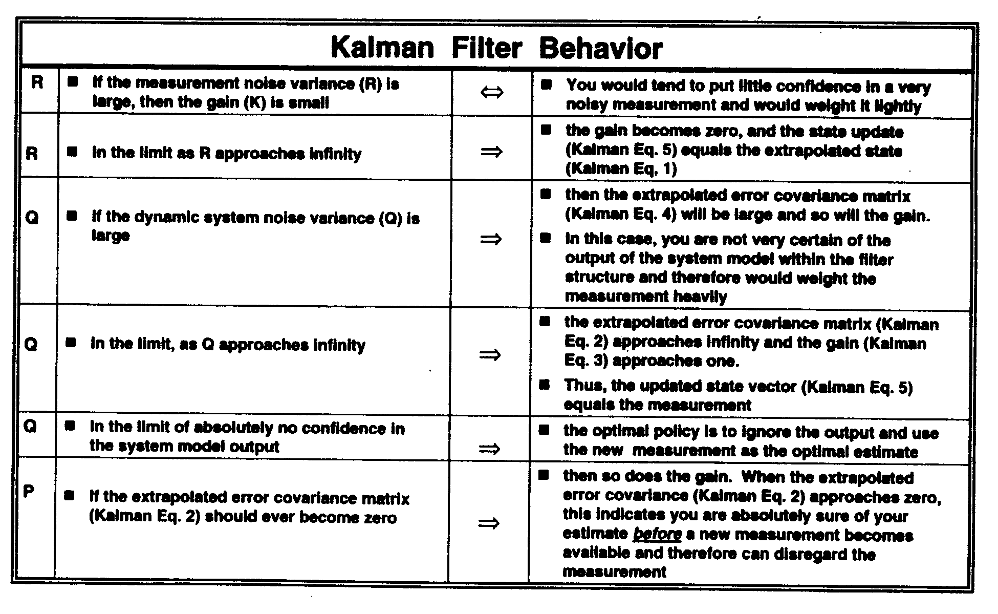
The five extended Kalman filter (EKF) equations are given in the below. They are called extended because the partial derivatives of the measurement with respect to the state variables is used in generating the measurement transformation matrix (H). The nomenclature above the various matrices indicate "prior to" or "after" a measurement vector has been incorporated. The overall "control" mechanisms for the Kalman filter are given in the table. The Kalman filter can be implemented in a variety of ways. Some include different coordinate frames such as polar or Cartesian, standard or square root formulations to handle single precision arithmetic processing systems, as well as the use of dedicated hardware boards that exploit the highly parallel arithmetic structure for purposes of order-of-magnitude processing speed.

Applications I have designed Kalman filters for include radar and infrared search and track (IRST) for both fire control on tactical aircraft and surveillance on surveillance platforms, electronic warfare (EW) related sensors such as electronic support measures (ESM) and missile warning receivers (MVM) for tactical aircraft, and ground- and airbased systems. The targets tracked include other airplanes, ground emitter sites, and missiles (surface-to-air [SAM], air-to-air [AAM], and ballistic). The application areas include both passive and active sensors and the limitations they bring in actual mission scenarios.

Some applications are considered unobservable in the estimation sense of the word. An example includes passive ranging of an airborne target. In this application, the use of angle-only data are used to estimate the range of the target airplane. Assuming the ownship (friendly aircraft) and target aircraft fly straight and level with constant velocities, range is unobservable (i.e., cannot be estimated). To turn the tracking problem into an observable one, the ownship must induce certain maneuvers. Namely, by inducing one derivative higher in its dynamics than the target aircraft range becomes observable. The ideal maneuver is the corkscrew where the observability capitalizes on the dimensional aspects of the problem at the same time. Many hours have led to very effective solutions to this problem. For the IRST application, the use of snake maneuvers with prescribed time-constraints and range estimation convergence limits were met.

Designing Kalman filters is an art, despite its strong theoretical and mathematical basis. Each application has its challenges. Common to all applications I have dealt with is the initialization of the error covariance matrix (P) and state vector (X). The more difficult problems are the passive sensor air-to-air applications - where angle-only measurements are available and when the measurement accuracy is poor. This forces the designer to make educated guesses of the target aircraft's range, speed and heading.

In some applications where the onboard sensor's detection range is well known, or the corridor where the target aircraft is approaching from is known, and target identification information is available, the "guessing" can be constrained. This applies to the passive time-to-interccpt (Tn) estimation for AAM's as well, where the additional unknown is the acceleration profile. In such difficult applications, the use of multiple model designs are useful. In essence, we run multiple Kalman filters in parallel and "blend" their results using a variety of methods. The idea behind this approach is to "capture" the spread of initial conditions and target dynamics possible. Although the approach requires considerably more processing intensive, its effectiveness is well worth its use.

In addition to the number of nice features cited in the second paragraph, the ability of the filter to give an estimate of how well (i.e., how accurate) its estimate is. For example, if the states are [x, xdot, y, ydot] and we desire to form the range estimate by taking the square root of the sums of squares, then by using the filter's updated error covariance and measurement transformation matrices, we can get the "accuracy" of this range estimate (i.e., standard deviation). The use of the filter's error bounds on the estimate is contingent upon the accuracy of the measurement and target dynamics models. Through the use of MATLAB simulation models, the sensitivity of the error bounds on uncertainties in these models can be examined a priori. For example, if the constant velocity, constant heading dynamics model is used and the target is accelerating instead, then the filter's error bounds may give a false value.

There are a host of design issues and lessons learned, but this is a good introduction. There are many books and hundreds of journal papers that the interested reader can investigate. If there are any questions or ideas, please feel free to write me. My e-mail address is: [e-mail address omitted]